Workshop setup

• Make sure you have an updated version of RStudio
• Install the code version-control system Git
• Create a Github account
• Run the following R command:

  install.packages(c("rmarkdown",
                      "htmlwidgets",
                      "bookdown",
                      "blogdown",
                      "DT",
                      "leaflet",
                      "rbokeh"))

• Be prepared to turn into a geek or just learn cool stuff

Exercice

1. Open RStudio
2. File > New File > R Markdown
3. Fill the fields author and title
4. Set default output format to HTML
5. Look at the source, then 🧶 Knit to HTML.

Try to identify these parts in the source and the output:

• The metadata
• The text
• The code
• The output

How does R Markdown work?

Metadata and options

Metadata with options are defined in the header of the .Rmd document as a set of key and value (YAML syntax).

---
output: html_document
---

---
output:
html_document:
    toc: true
  pdf_document:
    toc: false
---

Options available depend on the output. See ?html_document, ?pdf_document, ?word_document

Exercice

Edit the output options

Use ?html_document from your R console to:

1. Add a floating table of contents
2. Add a theme
3. Use the "kable" method to print data frames

🧶 Knit to HTML to see the output.

If this was easy, try to embed the Rmd source code to download.

Text style

# Header 1
## Header 2
### Header 3
#### Header 4
*italic* or _italic_
**bold**
`code`
```r
library(tibble)
data(iris)
glimpse(as_tibble(iris))
```

library(tibble)
data(iris)
glimpse(as_tibble(iris))

Lists

Lorem ipsum dolor sit amet,
consectetur
adipiscing elit.
- Cras convallis purus.
- Nunc faucibus.
- Maecenas ipsum dolor.
Nulla vehicula metus vel tortor
venenatis luctus.
Etiam tempus sit amet ligula
nec pretium. Aenean ultrices
massa sed pulvinar pulvinar.
1. Duis aliquam commodo volutpat.
1. Mauris ultrices.
1. Aliquam eu erat.

Images

![Hulk vs Trump](https://media.giphy.com/media/MkGyW2cOH7uhO/giphy.gif)

Links

[Hulk vs Trump](https://media.giphy.com/media/MkGyW2cOH7uhO/giphy.gif)
![Hulk vs Trump](https://media.giphy.com/media/MkGyW2cOH7uhO/giphy.gif)

Tables

| Time          | Session | Topic    |
|:--------------|:-------:|---------:|
| _left_        | _center_| _right_  |
| 01:00 - 01:50 | 1       | Anatomy  |
| 01:50 - 02:00 |         | *Break*  |
| 02:00 - 02:45 | 2       | Tables   |
| 02:45 - 03:00 |         | *Break*  |

• the : specify the alignement.
• Not convenient for long table, we will use instead to print the markdown table for us.

Chunks

This text is written in markdown
```{r}
library(tibble)
data(iris)
head(iris)
```

• r between brackets {}, why is that?
• Where is the code and the section?

Chunks

Code

library(tibble)
data(iris)
head(iris)

Print output

##   Sepal.Length Sepal.Width Petal.Length Petal.Width Species
## 1          5.1         3.5          1.4         0.2  setosa
## 2          4.9         3.0          1.4         0.2  setosa
## 3          4.7         3.2          1.3         0.2  setosa
## 4          4.6         3.1          1.5         0.2  setosa
## 5          5.0         3.6          1.4         0.2  setosa
## 6          5.4         3.9          1.7         0.4  setosa

Chunks

library(ggplot2)
data(iris)
ggplot(
      data=iris,
      aes(x = Sepal.Length,
          y = Sepal.Width)
  ) +
geom_point(
  aes(color=Species, shape=Species)
) +
xlab("Sepal Length") +
ylab("Sepal Width") +
ggtitle("Sepal Length-Width")

Chunks

library(leaflet)
leaflet(height=400, width=400) %>%
  addTiles() %>%
  addMarkers(lng=174.768, lat=-36.852,
             popup="The birthplace of R")

Map

+−

Leaflet | © OpenStreetMap contributors, CC-BY-SA

Chunks

library(rbokeh)
p <- figure() %>%
  ly_points(Sepal.Length, Sepal.Width,
    data = iris,
    color = Species, glyph = Species,
    hover = list(Sepal.Length, Sepal.Width))
p

Inline chunks

Syntax

We studied `r length(levels(iris$Species))` iris species and took measurements on `r nrow(iris)` flowers.

We found that Iris virginica had the longest sepal with a mean of `r mean(subset(iris,Species=="virginica")$Sepal.Length)` millimeters!

Output

This text is written in markdown.
We studied 3 iris species and took measurements on 150 flowers.
We found that Iris virginica had the longest sepal with a mean of 6.588 millimeters!

Chunks options

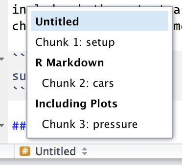
```{r dispIris, option1=value, option2=value}
library(tibble)
data(iris)
head(iris)
```

Chunk options

Chunk output can be customised with numerous options:

str(knitr::opts_chunk$get())

## List of 53
##  $ eval         : logi TRUE
##  $ echo         : logi TRUE
##  $ results      : chr "markup"
##  $ tidy         : logi FALSE
##  $ tidy.opts    : NULL
##  $ collapse     : logi FALSE
##  $ prompt       : logi FALSE
##  $ comment      : chr "##"
##  $ highlight    : logi TRUE
##  $ strip.white  : logi TRUE
##  $ size         : chr "normalsize"
##  $ background   : chr "#F7F7F7"
##  $ cache        : logi FALSE
##  $ cache.path   : chr "index_cache/html/"
##  $ cache.vars   : NULL
##  $ cache.lazy   : logi TRUE
##  $ dependson    : NULL
##  $ autodep      : logi FALSE
##  $ cache.rebuild: logi FALSE
##  $ fig.keep     : chr "high"
##  $ fig.show     : chr "asis"
##  $ fig.align    : chr "default"
##  $ fig.path     : chr "index_files/figure-html/"
##  $ dev          : chr "png"
##  $ dev.args     : NULL
##  $ dpi          : num 72
##  $ fig.ext      : NULL
##  $ fig.width    : num 7
##  $ fig.height   : num 7
##  $ fig.env      : chr "figure"
##  $ fig.cap      : NULL
##  $ fig.scap     : NULL
##  $ fig.lp       : chr "fig:"
##  $ fig.subcap   : NULL
##  $ fig.pos      : chr ""
##  $ out.width    : NULL
##  $ out.height   : NULL
##  $ out.extra    : NULL
##  $ fig.retina   : num 1
##  $ external     : logi TRUE
##  $ sanitize     : logi FALSE
##  $ interval     : num 1
##  $ aniopts      : chr "controls,loop"
##  $ warning      : logi TRUE
##  $ error        : logi FALSE
##  $ message      : logi TRUE
##  $ render       : NULL
##  $ ref.label    : NULL
##  $ child        : NULL
##  $ engine       : chr "R"
##  $ split        : logi FALSE
##  $ include      : logi TRUE
##  $ purl         : logi TRUE

Default options

```{r}
head(iris)
```

head(iris)

##   Sepal.Length Sepal.Width Petal.Length Petal.Width Species
## 1          5.1         3.5          1.4         0.2  setosa
## 2          4.9         3.0          1.4         0.2  setosa
## 3          4.7         3.2          1.3         0.2  setosa
## 4          4.6         3.1          1.5         0.2  setosa
## 5          5.0         3.6          1.4         0.2  setosa
## 6          5.4         3.9          1.7         0.4  setosa

Chunk option echo

```{r echo = FALSE}
head(iris)
```

##   Sepal.Length Sepal.Width Petal.Length Petal.Width Species
## 1          5.1         3.5          1.4         0.2  setosa
## 2          4.9         3.0          1.4         0.2  setosa
## 3          4.7         3.2          1.3         0.2  setosa
## 4          4.6         3.1          1.5         0.2  setosa
## 5          5.0         3.6          1.4         0.2  setosa
## 6          5.4         3.9          1.7         0.4  setosa

• Display results but not code.
• Useful to present results to people not interested by the code.
• Use echo = -1 to hide only the first line of a code chunk.

Chunk option eval

```{r eval = FALSE}
head(iris)
```

head(iris)

• Code is not evaluated.
• Useful to show exemple code.
• Use eval = -1 to evaluate every line of a code chunk except the first.

Chunk option include

```{r include = FALSE}
head(iris)
```

• Code is evaluated but no output (code, results and figures) is displayed.
• Useful in setup options and package installation.

Chunk option results

```{r results = "hold"}
1 + 1
2 + 2
```

1 + 1
2 + 2

## [1] 2
## [1] 4

• Hold all results in a code chunk and display them at the end.

Chunk option results

```{r results = "hide"}
1 + 1
ggplot(data = iris,
       aes(x = Petal.Length,
           y = Petal.Width)) +
  geom_point()
```

1 + 1
ggplot(data = iris,
       aes(x = Petal.Length,
           y = Petal.Width)) +
  geom_point()

Chunk options fig.height & fig.width

```{r fig.height = 3,
      fig.width = 5,
      echo = FALSE}
ggplot(data = iris,
       aes( x = Sepal.Length,
            y = Sepal.Width,
            color = Species)) +
  geom_point()
```

• width and height of the plot in inches
• Note that options are separated by commas

Chunk options

What output each option suppresses?

Table from R for Data Science

Global chunk options

Setup

You can change the default chunk options for all following chunks in your document.

```{r include = FALSE}
knitr::opts_chunk$set(
  collapse = TRUE,
  cache = TRUE,
  comment = "#>",
  fig.width = 6,
  fig.align = "center"
)
```

Exercice

Let's practice !

1. Open a new .Rmd document and run data(diamonds) within a chunk

2. Add the following text and fill it: We have data about XXXX diamonds. Only XXXX are larger than 2.5 carats.

3. Display all diamonds larger than 2.5 carats with the function DT::datatable().

4. Make an histogram of the carats. The figure should have an height and width of 4 inches.
5. DT::datatable() doesn't work with PDF or Word document, why?

Wrapping up

✔️ Document your document: use YAML to set up meaningful metadata

✔️ Style your document: use YAML to add options to your chosen output format

✔️ Organize your text: use markdown headers with #

✔️ Organize your code: use knitr chunk labels

✔️ Style your text: use markdown bold, italics, bullets, and lists

✔️ Style your output: use knitr chunk options

🧶 early, 🧶 often

Why using it?

Multiplateform | Portable | Reproducible

Impress your director with dynamic output | Turn into a geek | Expose your skills on the web

Launch document on the web

Mission

Send an HTML output on Github

Launch document on the web

5 steps

1. Open new GitHub repository and activate Github page
2. Link this new repo to a RStudio project
3. Add a .Rmd document and generate the HTML document (we know that part!)
4. Declare (add) and document (commit) the modifications on the repository
5. Send these modifications with the HTML output on Github via RStudio

Let's do it together!

Launch document on the web

1a. Open a new GitHub repository

• Name it as firstOnlineDocument
• Let's make the repository public

Launch document on the web

1b. Activate Github page

Launch document on the web

1b. Activate Github page

Launch document on the web

1b. Activate Github page

Several options

Launch document on the web

2. Link this new repo to a RStudio project

In RStudio: file > new project... > Version control > Git

• Fill the field Repository URL with the URL address of your repo and add .git at the end
• Exemple: https://github.com/SteveViss/firstOnlineDocument.git

Launch document on the web

3. Add a .Rmd document and generate the HTML document

• You know that part, so let's do it.
• We want to create a .Rmd and produces a .html file in the RStudio project folder.
• with the following filenames: index.html & index.Rmd
• Make sure you save the files within the project folder

Launch document on the web

4. Declare (add) and document (commit) the modifications on the repository

Launch document on the web

4. Declare (add) and document (commit) the modifications on the repository

Launch document on the web

5. Last step, send these modifications on the Github repo via RStudio

Launch document on the web

Wait few minutes and see the result at https://YOURUSERNAME.github.io/firstOnlineDocument/

The down universe

• Write a notebook: bookdown
• Write a thesis: thesisdown
• Write a scientific article rticles
• Create a poster: posterdown
• Create nice presentation: xaringan or rmarkdown
• Build a CV: vitae
• Generate a blog: blogdown
• Generate R package documentation: pkgdown

Motivation

1. Create a presentation
2. Use Markdown to quickly format your content
3. Insert code examples
4. Insert your R figures

Create a Rmarkdown presentation

Templates in R Studio

• ioslides
• slidy
• also "r presentations" but it uses a different markdown syntax so we won't present it here

Create a Rmarkdown presentation in R Studio

Create a Rmarkdown presentation in R Studio

ioslides

Specify the ioslides_presentation output format in the YAML metadata of your document

---
title: "My beautiful ioslide presentation"
author: "John Doe"
date: '2019-10-02'
output: ioslides_presentation
---

ioslides

Knit 🧶 to create the HTML presentation!

ioslides

Create new slides by using # or ##

# Section slides | super stuff

ioslides

Create new slides by using # or ##

# Section slide | with background image
{data-background=bg_mountain.jpg data-background-size=cover}

ioslides

Create new slides by using # or ##

## Slides with content
- I love science
- and **kitten!**
![](kitten.jpg){ width=60% }

ioslides - code

## Slide with R code
```{r, echo = TRUE}
fit <- lm(dist ~ 1 + speed, data = cars)
coef(summary(fit))
```

ioslides - plot

## Slide with R plot
```{r, echo = TRUE}
plot(dist ~ speed, data = cars)
```

ioslides - options

---
title: "My beautiful ioslide presentation"
author: "John Doe"
date: '2019-10-02'
output:
  ioslides_presentation:
    logo: insilecoLogo.png
---

ioslides - options

Customize

• presentation size using widesreen
• speed of slide transitions using transition
• incremental bullets using incremental
• text size using smaller

---
title: "My beautiful ioslide presentation"
author: "John Doe"
date: '2019-10-02'
output:
  ioslides_presentation:
    widescreen: true
    transition: slower
    incremental: true
    smaller: true
---

ioslides - Customization

You can customize your presentation by adding your own CSS and your own template

---
title: "My beautiful ioslide presentation"
author: "John Doe"
date: '2019-10-02'
output:
  ioslides_presentation:
    css: mystyles.css
    template: mytemplate.html
---

Slidy

To create a Slidy presentation in R studio

Slidy

• You can transform your ioslides presentation to a slidy presentation by changing the output format to slidy_presentation in the YAML
• Usage of slidy is similar to ioslides, but see details here

---
title: "My beautiful slidy presentation"
author: "John Doe"
date: '2019-10-02'
output: slidy_presentation
---

PowerPoint

• You can also generate a PowerPoint presentation using R!

---
title: "My beautiful PPT presentation"
author: "John Doe"
date: '2019-10-02'
output: powerpoint_presentation
---

Xaringan

• It is also possible to install R packages to create presentation
• ex: xaringan, see here and here

install.packages("xaringan")

---
title: "My beautiful Xaringan presentation"
subtitle: "Symposium"
author: "John Doe"
output:
  xaringan::moon_reader:
---
# Slide 1
wow!
---
# Slide 2
The end!

Xaringan

• QCBS R workshop presentations are built using xaringan!

Resources

1. R Markdown: The Definitive Guide - Chapter 4
2. ioslides
3. xaringan

Motivation

With Rstudio project

Bookdown - Examples

• Minimal: https://bookdown.org/yihui/bookdown-demo/

Bookdown - Examples

• Tufte style: https://bookdown.org/yihui/bookdown-demo3/

Bookdown - Usage

• Collection of .Rmd files
  • Individual chapter for each file
  • Chapter title defined by first-level heading #
  • Usual Rmarkdown syntax
  • Rendered by filename order by default

# Introduction
This is the introduction

# Chapter 1
This is the Chapter 1

# Conclusion
This is the conclusion

Bookdown - Usage

• Outputs options
  • HTML
  • pdf
  • E-Books

Bookdown - Getting started

Bookdown - Resources

• Github repository: https://github.com/rstudio/bookdown
• Bookdown book: https://bookdown.org/yihui/bookdown/

The down universe

• Write a notebook: bookdown
• Write a thesis: thesisdown
• Write a scientific article rticles
• Create a poster: posterdown
• Create nice presentation: xaringan or rmarkdown
• Build a CV: vitae
• Generate a blog: blogdown
• Generate R package documentation: pkgdown