Animations in R: Time series of erythemal irradiance in the St. Lawrence

July 5, 2017

  R plot animation NASA radiation St. Lawrence
  animation magrittr graphics plyr raster

David Beauchesne, Kevin Cazelles


The “need” for animations

As part of my PhD thesis, I am currently characterizing the intensity of multiple stressors in the estuary and gulf of St. Lawrence (see ResearchGate project for more details). I have recently needed (read: thought it would be cool) to create an animation of the temporal variations in ultra-violet intensity in the St. Lawrence. Here is how I did it.

Setting up R

R version used to build the last update of this post

1
2
sessionInfo()[[1]]$version.string
#R>  [1] "R version 4.2.0 (2022-04-22)"

Installing imagemagick

The package animation, which I used to create the animations in R, works with the application imagemagick, which can be installed using Homebrew on MacOS.

1
brew install imagemagick

Installing the package animation

1
`install.packages('animation', repos = 'http://yihui.name/xran')`

Data

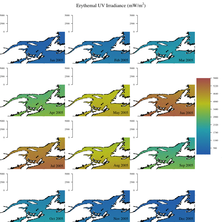
There is a incredible amount of data available on the NASA website. For this post, we downloaded all available data from NASA’s Ozone Monitoring Instrument (OMI) aboard the Earth Observing System’s (EOS) Aura satellite. More specifically, we used OMI/Aura Surface UVB Irradiance and Erythemal Dose Daily at a scale of 0.25 x 0.25 degree and selected the daily erythemal irradiance (mW/m2), i.e. the potentially harmful range of UV radiations, from October 1st 2004 to April 5th 2017. We then selected only the years with 12 months worth of data to create the following figures, i.e. from January 1st 2005 to December 31st 2016.

The maps generated in this post require the user to load ocean shapefile from Natural Earth.


 1
 2
 3
 4
 5
 6
 7
 8
 9
10
11
12
13
14
15
16
17
18
# UV data
UV <- readRDS('MonthOMI.rds')

# Projection
spatProj <- '+proj=longlat +ellps=WGS84 +datum=WGS84 +no_defs'

# Ocean shapefile
ocean <- readOGR(dsn = "shpfile", layer = "ne_10m_ocean") %>%
             spTransform(CRSobj = CRS(spatProj))
#R>  OGR data source with driver: ESRI Shapefile
#R>  Source: "/home/kc/git/inSilecoBlog/inSileco.github.io/content/post/2017/animationinR/shpfile", layer: "ne_10m_ocean"
#R>  with 1 features
#R>  It has 2 fields

class(ocean)
#R>  [1] "SpatialPolygonsDataFrame"
#R>  attr(,"package")
#R>  [1] "sp"

Set parameters and functions

We start be setting the different parameters and functions required to build the animation.

 1
 2
 3
 4
 5
 6
 7
 8
 9
10
11
12
13
14
15
16
17
18
19
20
21
22
23
24
25
26
27
28
29
30
31
32
# Graphical parameters
min_ <- min(UV[[1]], na.rm = TRUE) %>% plyr::round_any(., 100, floor) # Minimum values in UV dataset
max_ <- max(UV[[1]], na.rm = TRUE) %>% plyr::round_any(., 100, ceiling) # Minimum values in UV dataset
ext <- c(-72, -54, 44, 53) # c(xmin, xmax, ymin, ymax)
rbPal <- colorRampPalette(c('#2f6eb9','#2aadba','#c4c726','#b45f5f')) # color palette
labels <- matrix(seq(4,(151-4)), ncol = 12, nrow = 12,
  dimnames = list(2005:2016, month.abb), byrow = TRUE)  # Select only full years (start: 2004/10; end: 2017/04)

# Monthly trends
monthMean <- apply(X = UV[[1]], MARGIN = 3, FUN = mean, na.rm = TRUE) # monthly mean
monthSd <- apply(X = UV[[1]], MARGIN = 3, FUN = sd, na.rm = TRUE) # monthly sd
years <- 2005:2016
lowCI <- monthMean - (1.96*monthSd) # Lower confidence interval
upCI <- monthMean + (1.96*monthSd) # Upper confidence interval

# Empty plot function
eplot <- function(x = 1, y = 1, xmin = 0, xmax = 1, ymin = 0, ymax = 1) {
  plot(x = x, y = y, bty = "n", ann = FALSE, xaxt = "n", yaxt = "n",
    type = "n", bg = 'grey', ylim = c(ymin, ymax), xlim = c(xmin, xmax))
}

# Legend function
colorBar <- function(colRamp, min, max, nticks = 11, ticks = seq(min, max, len = nticks)) {
    scale = (length(colRamp) - 1) / (max - min)
    par(mar = c(5,0.5,5,4))
    plot(c(0,10), c(min_, max_), type = 'n', bty = 'n', xaxt = 'n', xlab =' ', yaxt = 'n', ylab = '')
    axis(4, ticks, las = 1, cex = 1.5)
    for (i in 1:(length(colRamp) - 1)) {
        y = (i - 1) / scale + min
        rect(0, y, 10, y + 1 / scale, col = colRamp[i], border = NA)
    }
}

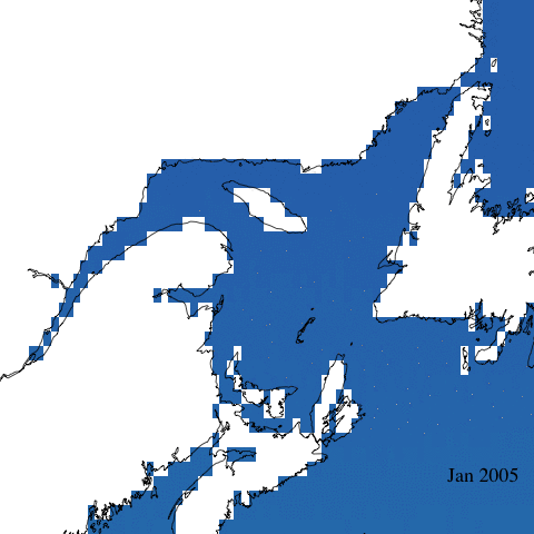
Create first animation

Let’s start with a simple animation of erythemal irradiance for 2005.

 1
 2
 3
 4
 5
 6
 7
 8
 9
10
11
saveGIF({
  for(i in 1:ncol(labels)){
      par(mar = c(0,0,0,0), pch = 21,  xaxs = "i", yaxs = "i", family = "serif")
      r <- raster::raster(UV[[1]][,,labels[1,i]], xmn = ext[1], xmx = ext[2], ymn = ext[3], ymx = ext[4], crs = spatProj) %>%
          mask(ocean)
      eplot(xmin = ext[1], xmax = ext[2], ymin = ext[3], ymax = ext[4])
      plot(r, col= rbPal(100), breaks = seq(min_,max_,length.out=100), legend = FALSE, add = TRUE)
      plot(ocean, add = TRUE, lwd = 2)
      text(x = -54.5, y = 45, labels = paste(colnames(labels)[1], rownames(labels)[i]), adj = 1, cex = 1.5)
  }
}, movie.name = "UV2005animate.gif")

Create complex animation

Now let’s make a more informative and complex animation that allows to visualize monthly erythemal irradiance through the years as well as annual trends.

 1
 2
 3
 4
 5
 6
 7
 8
 9
10
11
12
13
14
15
16
17
18
19
20
21
22
23
24
25
26
27
28
29
30
31
32
33
34
35
36
37
38
39
40
41
42
43
44
45
46
47
48
ani.options(ani.height = 720, ani.width = 720)
saveGIF({
    for(i in 1:nrow(labels)) {
        #layout
            mat <- matrix(c(13:15, 1:3, 16:18, 4:6, 19:21, 7:9, 22:24, 10:12),
              ncol = 3, nrow = 8, byrow = TRUE) %>%
                  cbind(c(0, 0, 25, 25, 25, 25, 0, 0)) %>%
                  rbind(26, .)
            layout(mat, widths = c(3, 3, 3, 1.25), heights = c(1, rep(c(2, 3), 4)))

        # Rasters
            for(j in 1:ncol(labels)) {
                par(pch = 21,  xaxs = "i", yaxs = "i", family = "serif", mar = c(0,0,0,0))
                r <- raster::raster(UV[[1]][,,labels[i,j]], xmn = ext[1], xmx = ext[2],
                    ymn = ext[3], ymx = ext[4], crs = spatProj) %>%
                      mask(ocean)
                eplot(xmin = ext[1], xmax = ext[2], ymin = ext[3], ymax = ext[4])
                image(r, col= rbPal(100), breaks = seq(0,max_,length.out = 101), legend = FALSE, add = TRUE)
                plot(ocean, add = TRUE)
                text(x = -54.5, y = 45, labels = paste(colnames(labels)[j], rownames(labels)[i]), adj = 1, cex = 1.5)
            }

        # Plot trends
            for(j in 1:ncol(labels)) {
                temporal <- data.frame(years = years[1:i], monthMean = monthMean[labels[1:i, j]],
                    lowCI = lowCI[labels[1:i, j]], upCI = upCI[labels[1:i, j]]) %>%
                            na.omit()
                polyY <- c(temporal$upCI, rev(temporal$lowCI)) # Y coordinates for confidence interval polygon
                polyX <- c(temporal$years, rev(temporal$years)) # X coordinates for confidence interval polygon

                par(mar = c(0,3,1,1), family = "serif")
                eplot(xmin = 2005, xmax = 2016, ymin = 0, ymax = max(upCI))
                polygon(polyX, polyY, border = 'transparent', col = "#d9e5f4")
                lines(temporal$monthMean ~ temporal$years, lwd = 0.5, col = '#0057bb')
                axis(side = 2, at = seq(0, plyr::round_any(max(upCI), 1000, ceiling), by = 2500),
                  las = 1, pos = 2004.75, cex =  1.5)
            }

        # Plot legend
            colorBar(rbPal(101), min = 0, max = max_)

        # Graph title
            par(mar = c(0,0,0,0))
            eplot(xmin = 0, xmax = 10, ymin = 0, ymax = 10)
            text(x = 5, y = 5, labels = bquote("Erythemal UV Irradiance (mW/m" ^2 *")"), cex = 2)

    }
}, movie.name = "UVanimate.gif")

Concluding remarks

As you can see, it is quite straightforward to create powerful and informative animations in R.

Session info

 1
 2
 3
 4
 5
 6
 7
 8
 9
10
11
12
13
14
15
16
17
18
19
20
21
22
23
24
25
26
27
28
29
30
31
32
33
34
35
36
37
38
39
40
41
42
43
sessionInfo()
#R>  R version 4.2.0 (2022-04-22)
#R>  Platform: x86_64-pc-linux-gnu (64-bit)
#R>  Running under: Debian GNU/Linux bookworm/sid
#R>  
#R>  Matrix products: default
#R>  BLAS:   /usr/lib/x86_64-linux-gnu/blas/libblas.so.3.10.1
#R>  LAPACK: /usr/lib/x86_64-linux-gnu/lapack/liblapack.so.3.10.1
#R>  
#R>  locale:
#R>   [1] LC_CTYPE=en_US.UTF-8       LC_NUMERIC=C              
#R>   [3] LC_TIME=en_US.UTF-8        LC_COLLATE=en_US.UTF-8    
#R>   [5] LC_MONETARY=en_US.UTF-8    LC_MESSAGES=en_US.UTF-8   
#R>   [7] LC_PAPER=en_US.UTF-8       LC_NAME=C                 
#R>   [9] LC_ADDRESS=C               LC_TELEPHONE=C            
#R>  [11] LC_MEASUREMENT=en_US.UTF-8 LC_IDENTIFICATION=C       
#R>  
#R>  attached base packages:
#R>  [1] stats     graphics  grDevices utils     datasets  methods   base     
#R>  
#R>  other attached packages:
#R>  [1] rgdal_1.5-32           plyr_1.8.7             raster_3.5-15         
#R>  [4] sp_1.4-7               magrittr_2.0.3         animation_2.7         
#R>  [7] inSilecoRef_0.0.1.9000
#R>  
#R>  loaded via a namespace (and not attached):
#R>   [1] Rcpp_1.0.8.3      lattice_0.20-45   lubridate_1.8.0   ps_1.7.0         
#R>   [5] assertthat_0.2.1  digest_0.6.29     utf8_1.2.2        mime_0.12        
#R>   [9] R6_2.5.1          backports_1.4.1   evaluate_0.15     httr_1.4.3       
#R>  [13] blogdown_1.10     pillar_1.7.0      rlang_1.0.2       curl_4.3.2       
#R>  [17] data.table_1.14.2 miniUI_0.1.1.1    callr_3.7.0       jquerylib_0.1.4  
#R>  [21] DT_0.23           rmarkdown_2.14    RefManageR_1.3.0  rcrossref_1.1.0  
#R>  [25] stringr_1.4.0     htmlwidgets_1.5.4 igraph_1.2.11     shiny_1.7.1      
#R>  [29] compiler_4.2.0    httpuv_1.6.5      xfun_0.31         pkgconfig_2.0.3  
#R>  [33] htmltools_0.5.2   tidyselect_1.1.2  tibble_3.1.7      httpcode_0.3.0   
#R>  [37] bookdown_0.26     codetools_0.2-18  fansi_1.0.3       crayon_1.5.1     
#R>  [41] dplyr_1.0.9       withr_2.5.0       later_1.3.0       grid_4.2.0       
#R>  [45] crul_1.2.0        jsonlite_1.8.0    xtable_1.8-4      lifecycle_1.0.1  
#R>  [49] DBI_1.1.2         cli_3.3.0         stringi_1.7.6     promises_1.2.0.1
#R>  [53] xml2_1.3.3        bslib_0.3.1       ellipsis_0.3.2    targets_0.12.0   
#R>  [57] generics_0.1.2    vctrs_0.4.1       tools_4.2.0       glue_1.6.2       
#R>  [61] purrr_0.3.4       processx_3.5.3    fastmap_1.1.0     yaml_2.3.5       
#R>  [65] terra_1.5-21      base64url_1.4     knitr_1.39        sass_0.4.1

Edits

Apr 27, 2022 -- Beautify the code and archive the post.